Locking & Unlocking Cells in a Range

In this post, I am going to show you how to lock and unlock cells using Conditional Formatting and VBA.

Why did I need this?

One of the improvements for the Student_Timesheet_Tool.xlsm was to prevent data entry in dates that were not in the selected period. The previous file allowed data entry in every cell; it was even possible to delete formulas. This was a feature that I knew I wanted to address.

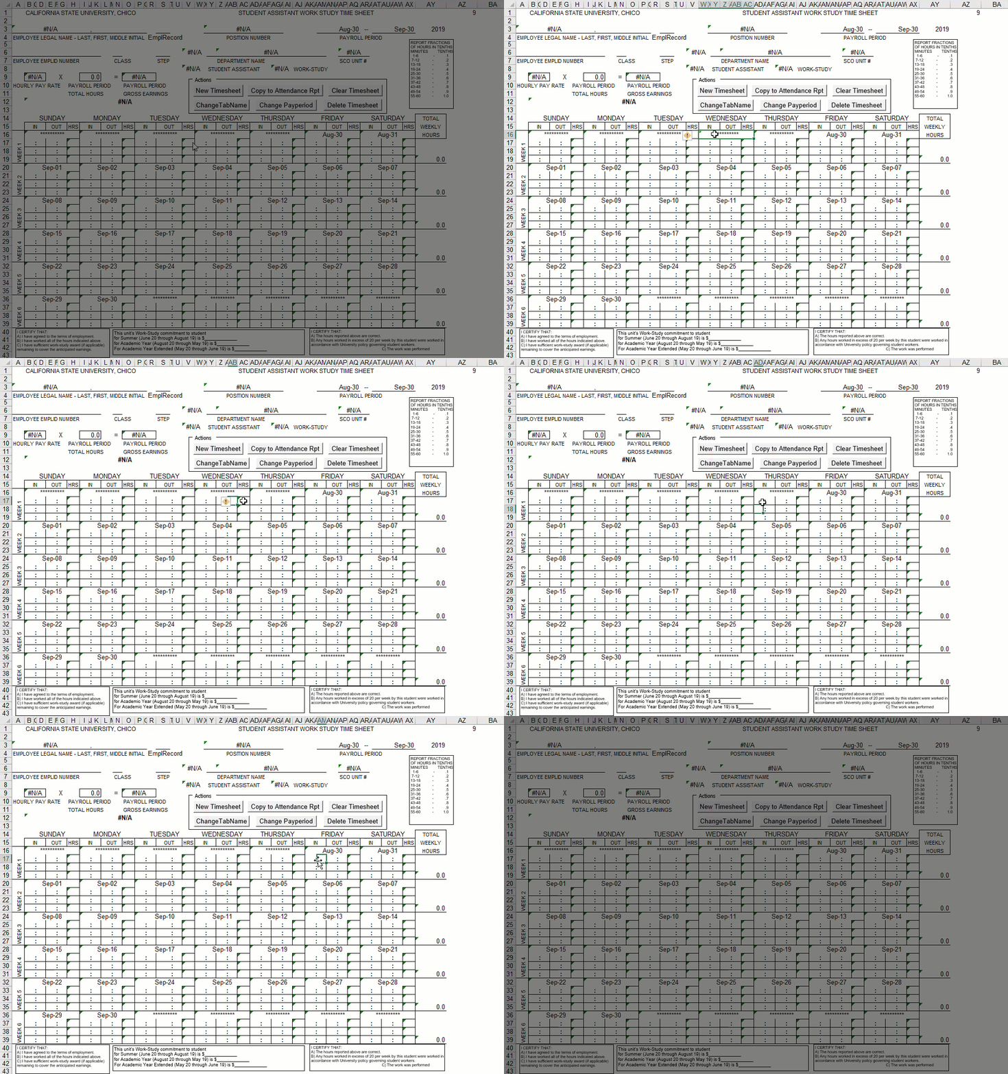
The Goal

The new improved file would only allow users to enter/modify data in the cells which I allow. The dynamic nature of this feature is actually pretty in depth but, I will show the foundation for the solution.

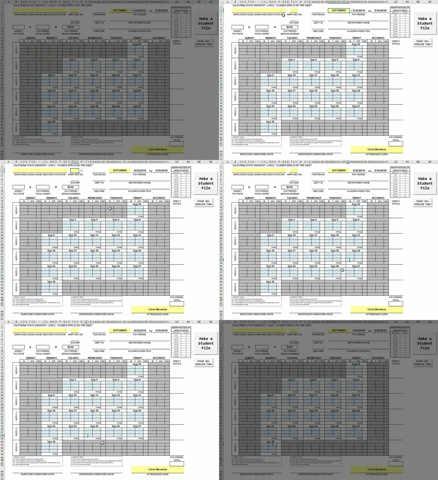
Setting the base background color

In the calendar matrix, data entry should only occur in cells designated either ‘IN’ or ‘OUT’. For each of those cells, I decided to fill them in Aqua.

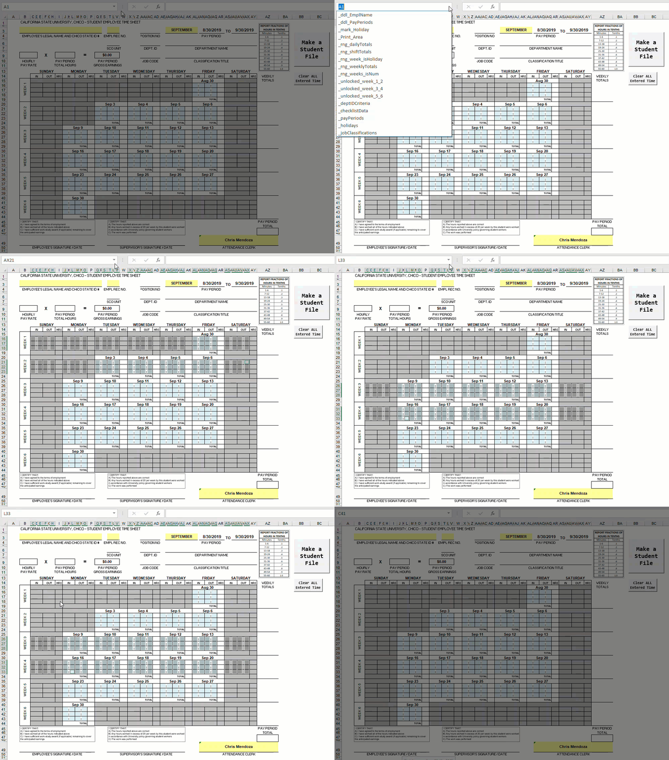
Not only are each of these named ranges filled Aqua, they are also unlocked in Format Cells > Protection.

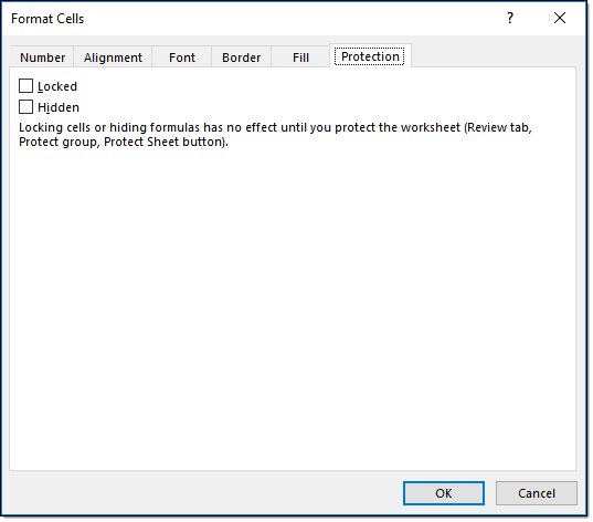
Every other cell in the worksheet that is not Yellow or Aqua is ‘Locked’ in Format Cells > Protection.

VBA Code

Visually filling the cells Aqua, or some other color, actually has a really important role in this locking and unlocking of cells. Without the color, how would you tell Excel which cells need to be locked and unlocked? This is how I told Excel what to do.

Public Sub LockCells()
    currentSheetName = ActiveSheet.Name
    Dim rng As Range: Set rng = Worksheets(currentSheetName).Range("C15:AY44")
    Dim cel As Range

    'colorIndex = 15 - White, Background 1, Darker 25%
    'colorIndex = 20 - Aqua, Accent 5, Lighter 80%
    
    Worksheets(currentSheetName).Unprotect Password:="SuperSecretPassword"
    For Each cel In rng.Cells
        With cel
            If .DisplayFormat.Interior.colorIndex = 15 Then
                .Locked = True
            ElseIf .DisplayFormat.Interior.colorIndex = 20 Then
                .Locked = False
            End If
        End With
    Next cel
    Worksheets(currentSheetName).Protect Password:="SuperSecretPassword", userinterfaceonly:=True
End Sub

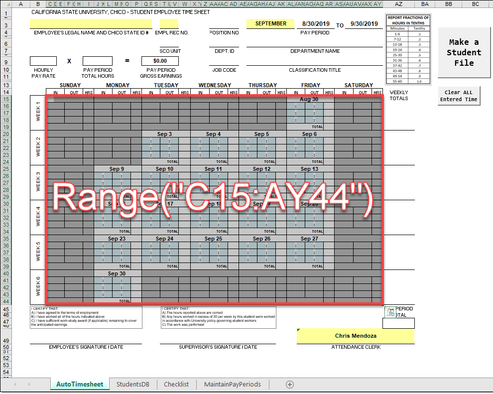
colorIndex = 15 is the Gray and colorIndex = 20 is the Aqua color. So the base color is always Aqua and the Gray color comes from plain old conditional formatting that I’ll talk about in a bit. The .Locked = true is the same as you checking the box in the Format Cells dialog.

Conditional Formatting

Before we can talk about the Conditional Formatting rules I have to explain a little bit about how the dates are generated/displayed. Using the period ‘SEPTEMBER’ as an example:

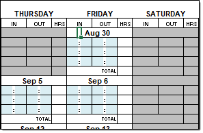
=IF(
  $AN$1="**********",
  IF(
    AF15="**********",
    IF(
      WEEKDAY($AN$3)=6,
      $AN$3,
      "**********"
    ),
    AF15+1
  ),
  IF(
    WEEKDAY($AN$1)=6,
    $AN$1,
    AF15+1
  )
)

Basically, our need for understanding in this post is, is this value an integer. If it is, we do something, if it is not, we do something else.

So let’s find out if what is returned is an integer or not.

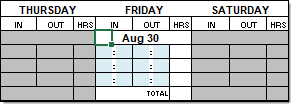
=IF(ISNUMBER(AM15),1,0)

If AM15 is a number, return 1, otherwise 0. Remember a date is an integer. Incidentally, you’re not seeing either the 1 or 0 because I have changed the font color to white.

Ok, now the Conditional Formatting

For each date range I wrote conditional formatting to check whether or not a 1 or 0 exists.

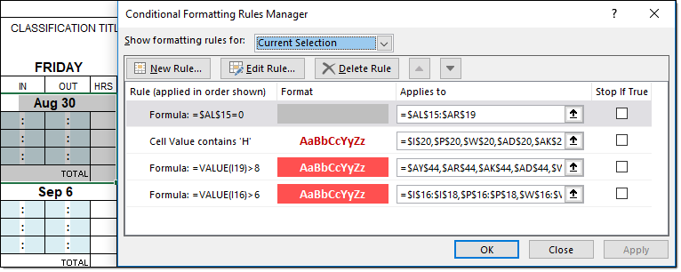
Can you see how that works?

The Result

The Sub LockCells () gets called in a Private Sub Worksheet_Change () event, the drop down selection change making the locking and unlocking of cells dynamic.